When items are on sale, it's often not until you get to the checkout before you discover just how much a 15 or 20 percent discount is saving you. With Microsoft Excel 2013, you can quickly calculate the savings on numerous items using any discount percentage.
If you already know two values, you can use Excel to calculate the percentage difference between those numbers, too. For example, you can calculate the percentage your savings account has grown in a month, or how much weight you have gained or lost since the last time you weighed yourself.
Video of the Day
Video of the Day
Calculating Percentage Discount Savings
Step 1
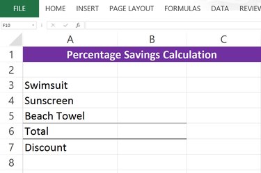
Open a new blank workbook in Excel. Enter some items in Column A that are being discounted. Beneath those items in Column A, add the words "Discount" and then "Total." Enter the normal price beside each item in column B.
Step 2
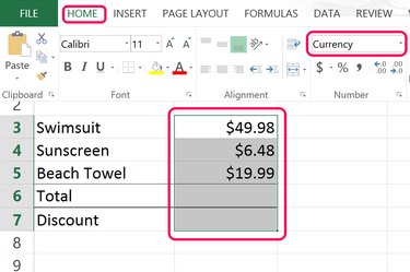
Highlight the cells in Column B by dragging the cursor over them. Click the "Home" tab and select "Currency" from the Ribbon's Number menu.
Step 3
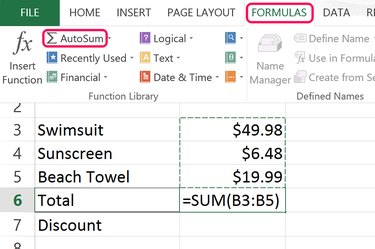
Click the empty cell in Column B beneath the prices, which is also beside the word "Total." Click the "Formulas" tab and then click "Autosum" in the Ribbon. Press "Enter." The Autosum formula adds all of the numbers in the column and gives you the total price of your items.
Step 4
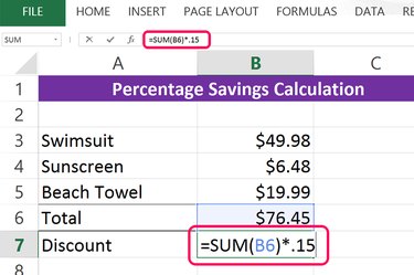
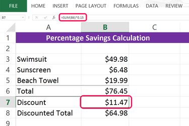
Click the cell beneath the total in Column B to calculate the percentage savings. Type the following formula in the cell, replacing "B6" with the cell number containing your total and replacing ".15" with the percentage of your discount: =SUM(B6)*.15
There are four aspects to this formula. a) The formula begins with =SUM. b) The cell number is placed in brackets, such as (B6). c) The asterisk represents a multiplication sign in Excel. d) The percentage is expressed as a decimal.
In our example, the total is in cell B6. The discount is 15 percent, so this is expressed as 0.15.
Step 5
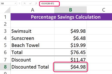
Calculate the total discounted price by subtracting the discount from the total. Type the following formula, replacing "B6" with your total's cell number and "B7" with your discount cell number: =SUM(B6-B7)
Because the values you are subtracting are both cell numbers, they go in the same set of parentheses.
Calculating Percentage Change in Two Numbers
Step 1
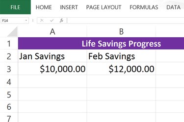
Type two numbers in an Excel worksheet. For example, to calculate the increase in a savings account between two months, type one month's savings total in cell A3 and the next month's total in cell B3.
Step 2
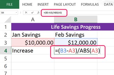
Click on any cell in the worksheet where you want the percentage change to appear. The formula for this operation has two components. First, you need Excel to subtract the first number from the second number to find the difference between them. Secondly, Excel needs to divide this difference by the first value. For example, if your savings account went from $10,000 to $12,000 in one month, the difference is $2,000. Dividing $10,000 by $2,000 gives you the percentage difference of 20 percent.
Type the following formula in the cell and press "Enter," replacing "A3" with the cell containing your first value and "B3" with the cell containing your second number:
=(B3-A3)/ABS(A3)
The "ABS" function is used in this formula in case the difference between the two values is a negative number. ABS converts a negative number to an absolute, or positive, number.
Step 3
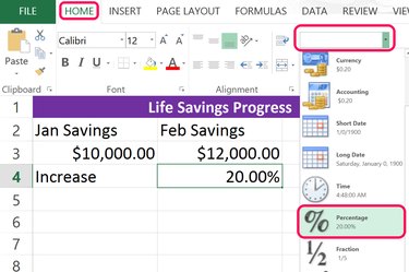
Click the "Home" tab and click the "Format" menu, located in the Number section of the Ribbon. Select "Percentage" from the drop-down menu.